Frank Jin

Project 4: Stitching and Panoramics

In this project I continue to use keypoint matching to transform images in interesting ways. This project focuses on stitching multiple images together forming a single panoramic image.

Step 1: Recovering Homographies

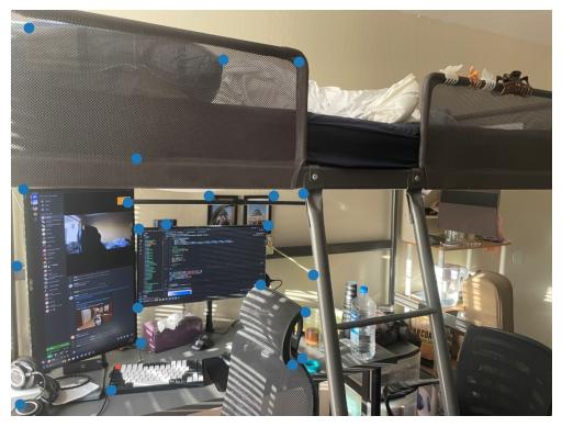
The first step in the stitching process is to compute the transform between the point-correspondances we manually define. We have to solve for 8 degrees of freedom so to get a solution we need 4 points. However, defining exactly 4 points may lead to a poor transform if there is noise. Hence we can define more than 4 points to mitigate the effect of noise. However, this leads us to a over-constrained solution. We can solve this by using least squares to solve for the variables we need.

After solving, we can use this the transformation matrix to transform our image so that the keypoints line up with one another. In this step, I noticed that keypoints that are more spread out in the image tend to work better than clustered keypoints, the edges of the images where keypoints were clustered would be warped out of shape. I suspect this is because when doing least squares, clustered keypoints are much more effected by noise even when taking multiple samples since a small variation will cause large changes. I imagine this to be like trying to line up two pieces of paper use the corners versus using a box inside the paper. Obviously lining up the paper's corners will product much accurate results.

This method, however, left some bright lines between the transformed triangles. I believe this is due to the transformation overlapping the triangles together at random locations, since the pixles are brighter intensity but the correct hue. This resulted in it being very difficult to debug, in the future, another method like direct pixle interpolation may provide better results.

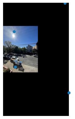
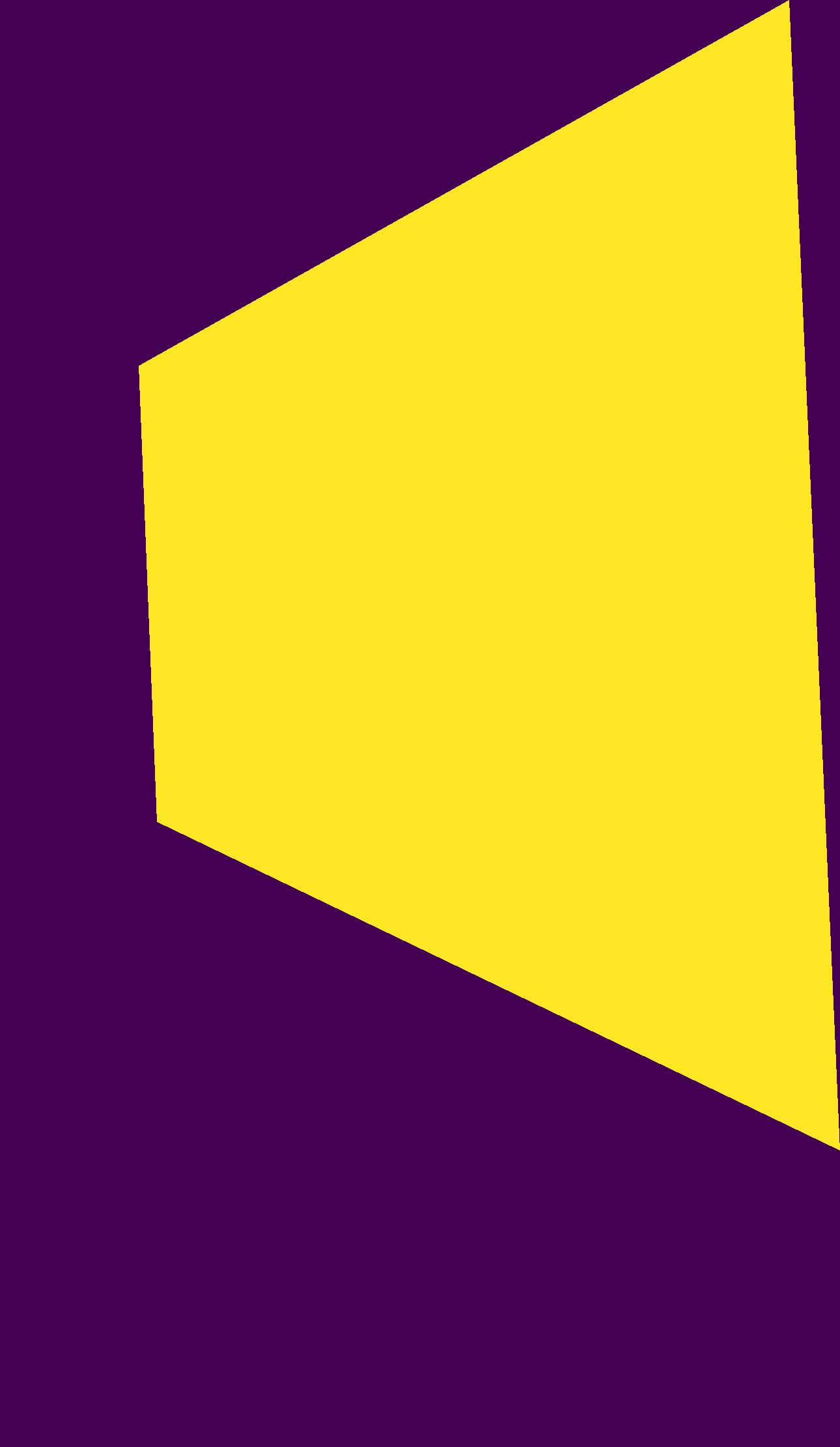
After the warp has been calculated, I warp the image corners. Since some of them may end up as negative coordinates, I pad and shift the image that I am alligning to. Then using the shifted warped corners, I create a mask by drawing a filled polygon using the PIL library. This shifted mask is used to specify the coordinates to fill relative to the padded image. The mask is then unshifted to find the coordinates to fill relative to the original image, these points are then put through the interpolator to calculate the values for each pixel. The pixle values are then applied according to the shifted mask.

Padded and Shifted

Shifted Mask

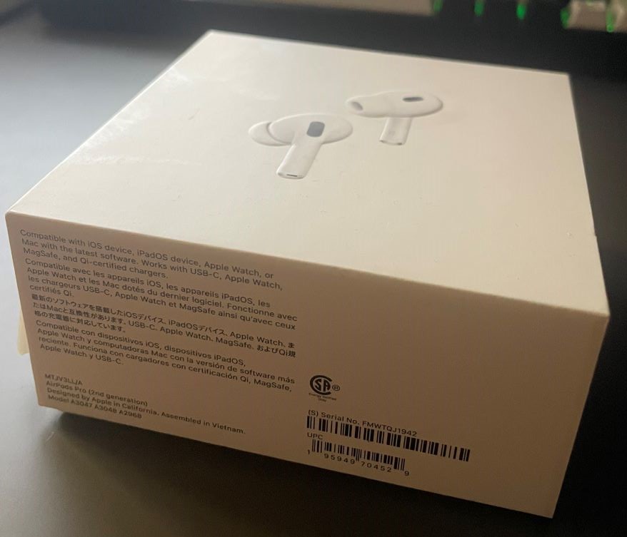
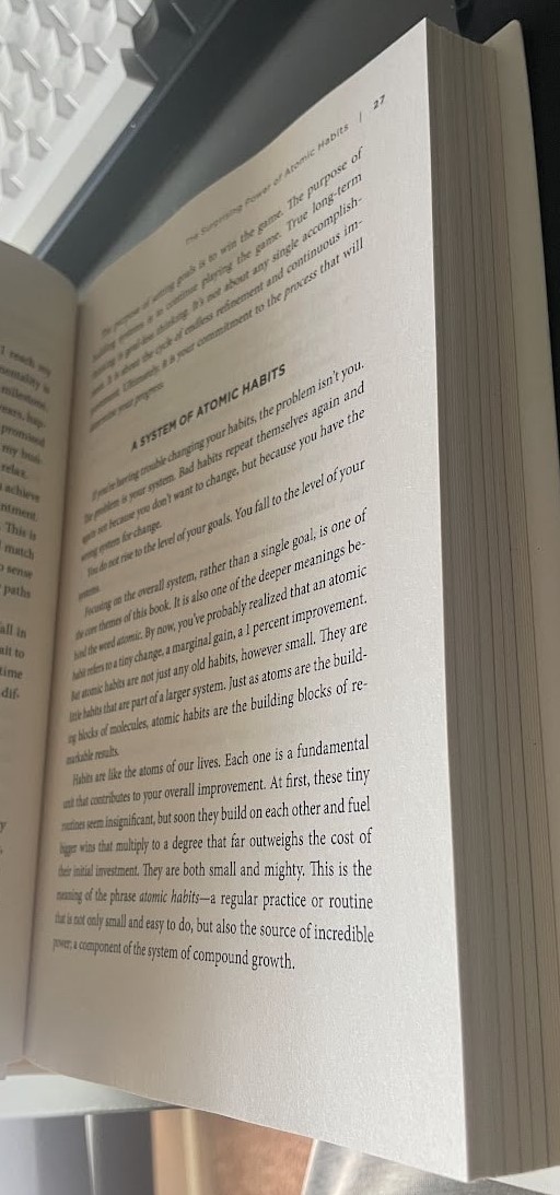
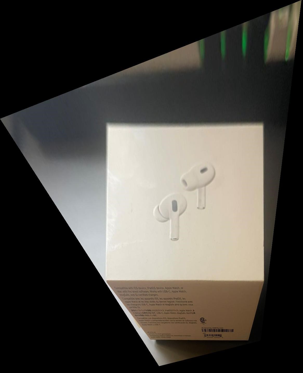
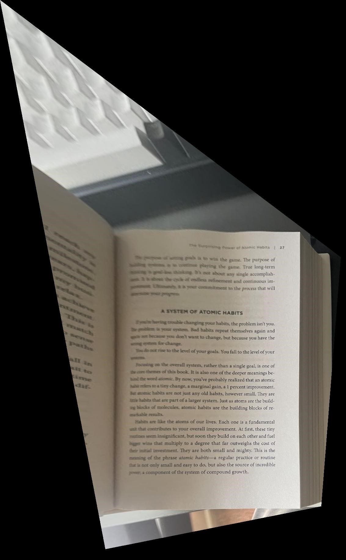
Finally with the setup being done, we can go onto shifting some images. First off is rectifying images. This was not too bad, as we just have to manually define the rectangular points we want our subject to warp into, and make a dummy second image (a zero value image in my case). However, due to only having 4 points and the large skew of some of the images, warping the corners would sometimes give extremely large coordinate values. The work around for this was to just crop the image to be as close to the subject as possible, therefore minimizing the coordinates of the warped corners. I also tried warping something with text on it to see if the text could be read after warping. The result was that the text could be read, however, with a camera with better depth of view I believe the results would be better.

Box

Book

Box Rectified

Book Rectified

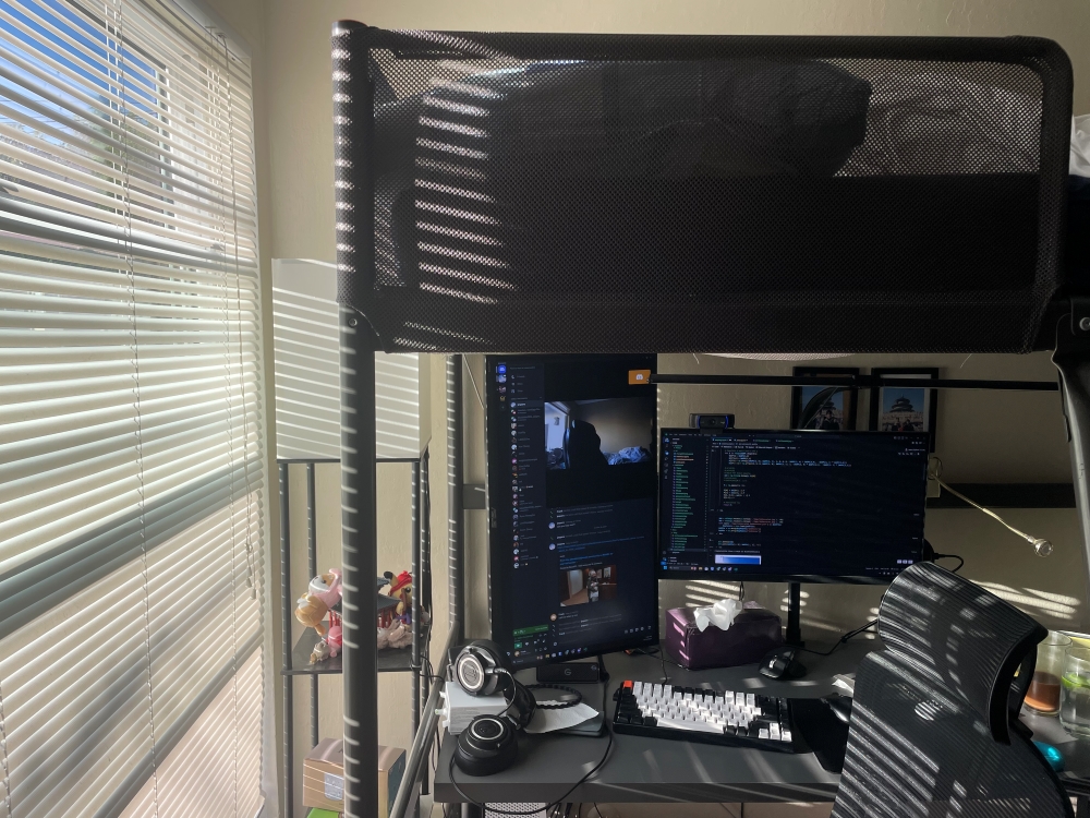
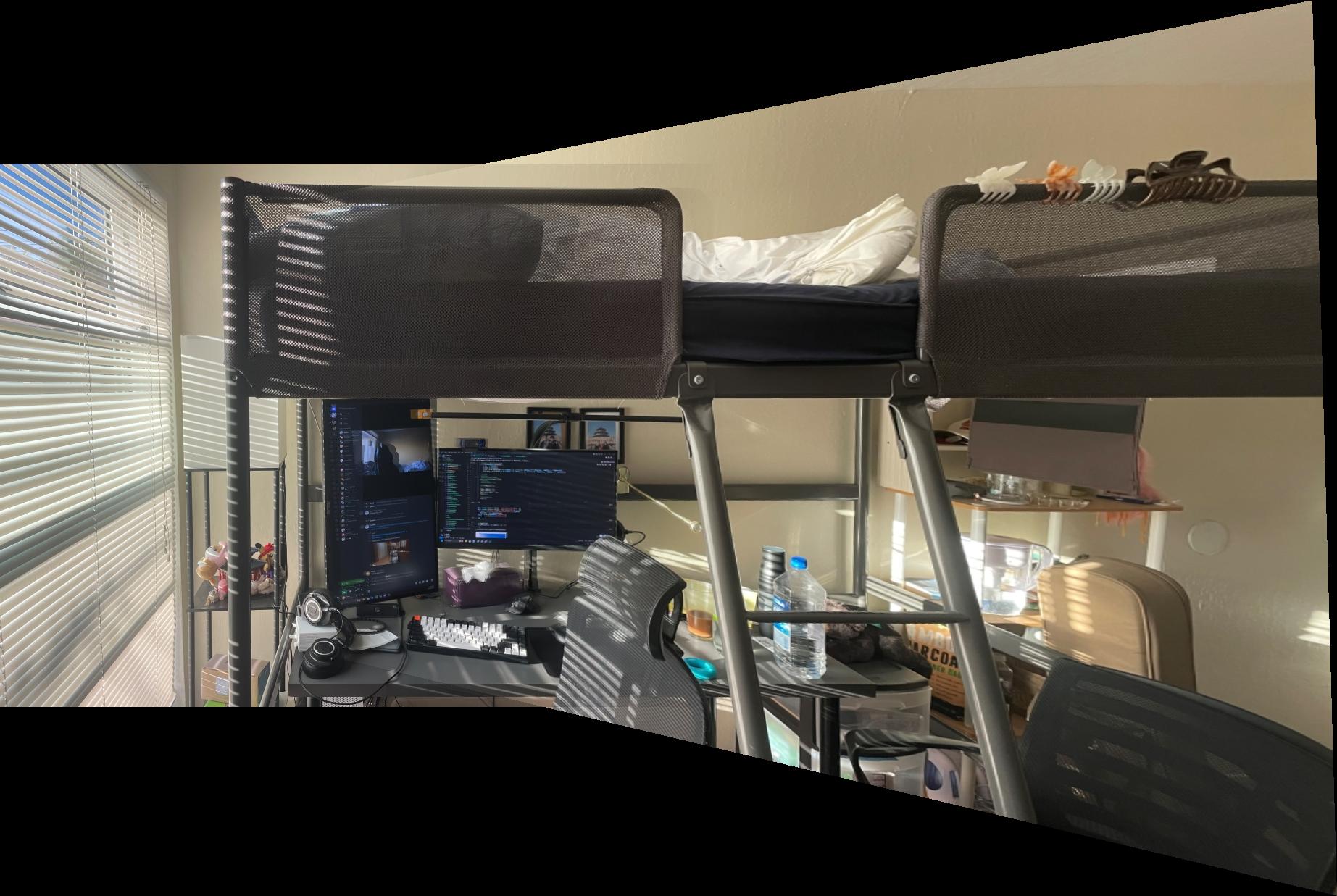
It is a relatively easy transition to go from this, to stitching images together. Its here where I ran into the issue with the point-correspondances clustering problem. In the example below, you see that objects on the edges of the stitch do not line up properly even with blending on overlaps due to most of the points defined being in near the monitor area. Another issue is that due to the camera autoadjusting contrast, brightness, etc, the edges of the two frames become very obvious, so its apparent a better blending method is needed.

Bedroom: Img 1

Bedroom Correspondances: Img 2

Bedroom Pano with Average blending

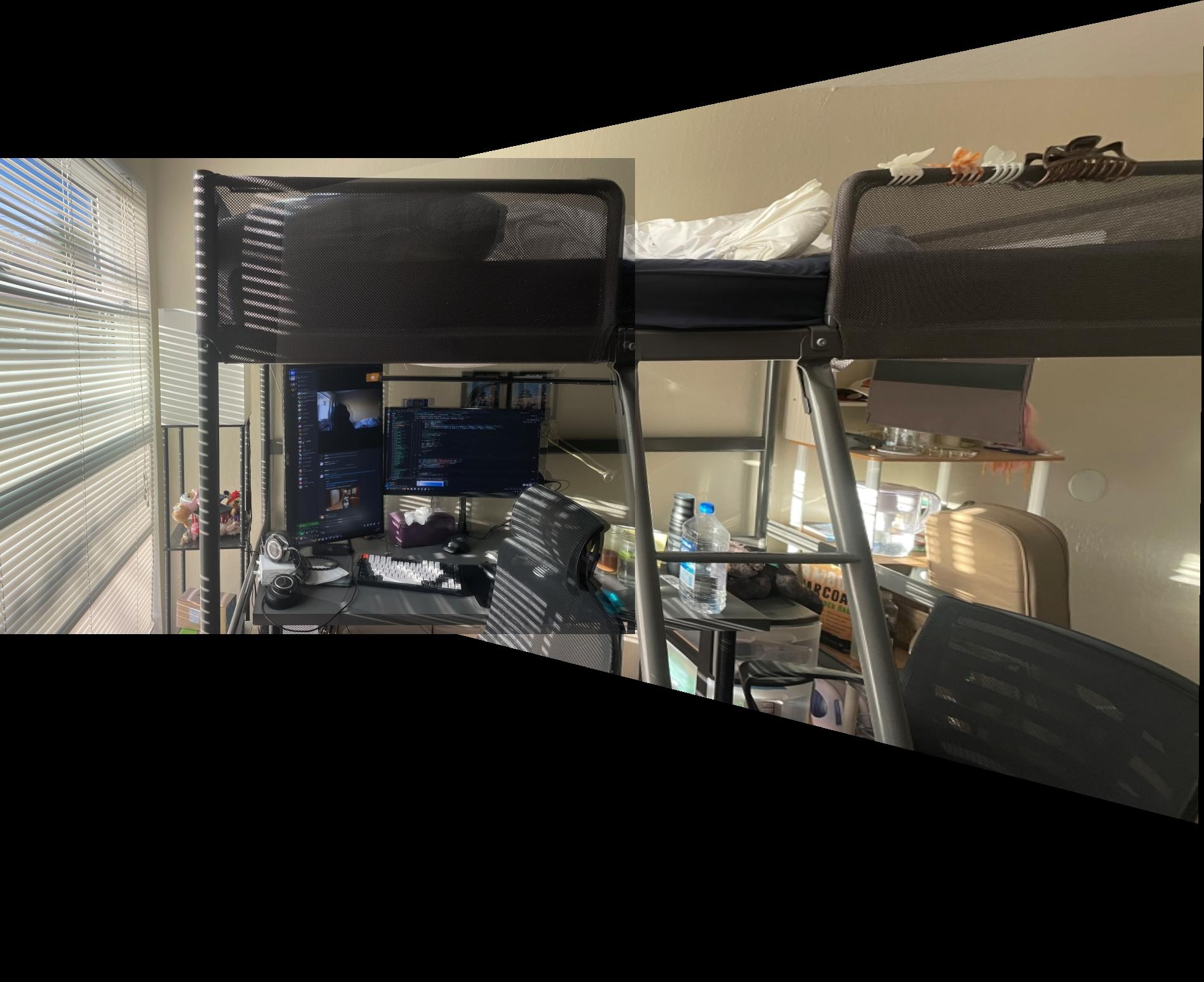
I tried again but this time I blended the images according to their x-pixel (Bell and Whistle?) coordinates and made sure to pick an image where more points could be determined on the edges. Even here, the wires and the sky were not ideal since they didnt have many identifiable features.

Outside: Img 1

Outside Correspondances: Img 2

Outside Pano with Average Blending

Outside Pano with X-cord blending

As you can see the x-coord blending works much better, and the artifacts are mostly gone. I also attempted x and y coordinate blending, however due to the way pixels values are set, it makes it difficult to calculate a smooth scaling array for both the x and y directions.

Here is another example:

Tree Correspondances: Img 1

Tree: Img 2

Outside Pano with Average Blending

Automatic Point-Correspondances

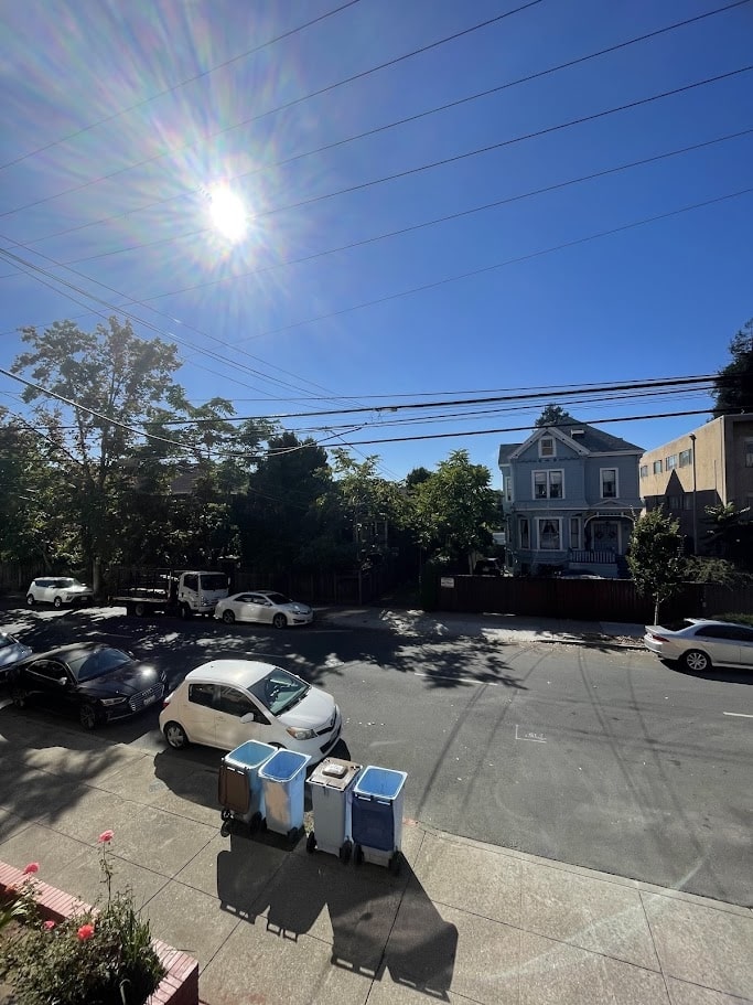
Instead of the manual trudge of defining points, we can also try to use an algorithmic approach. In this section we try to do exactly that. We will be going through the pipeline with these images.

Starter Images

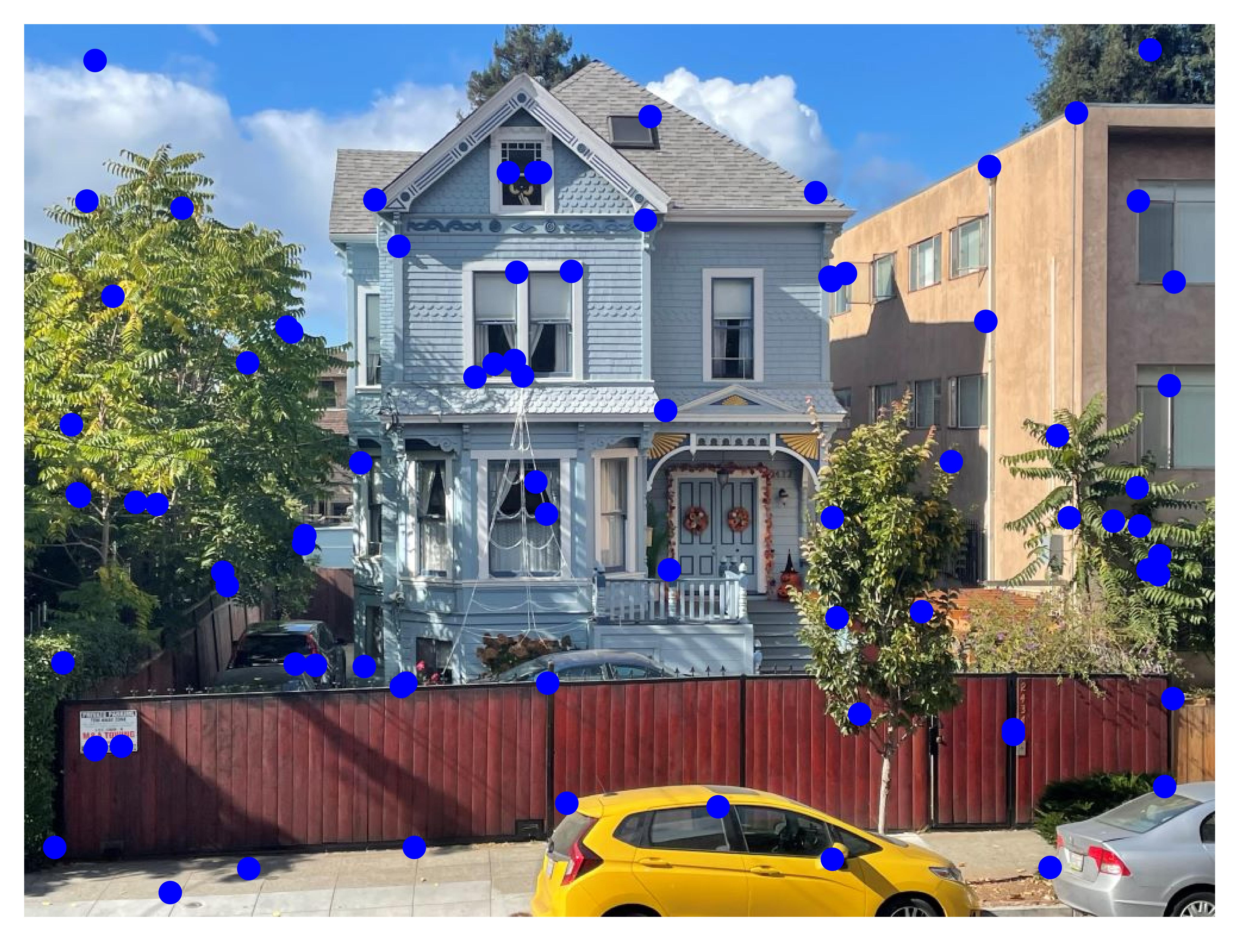
Harris Corners

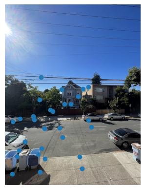
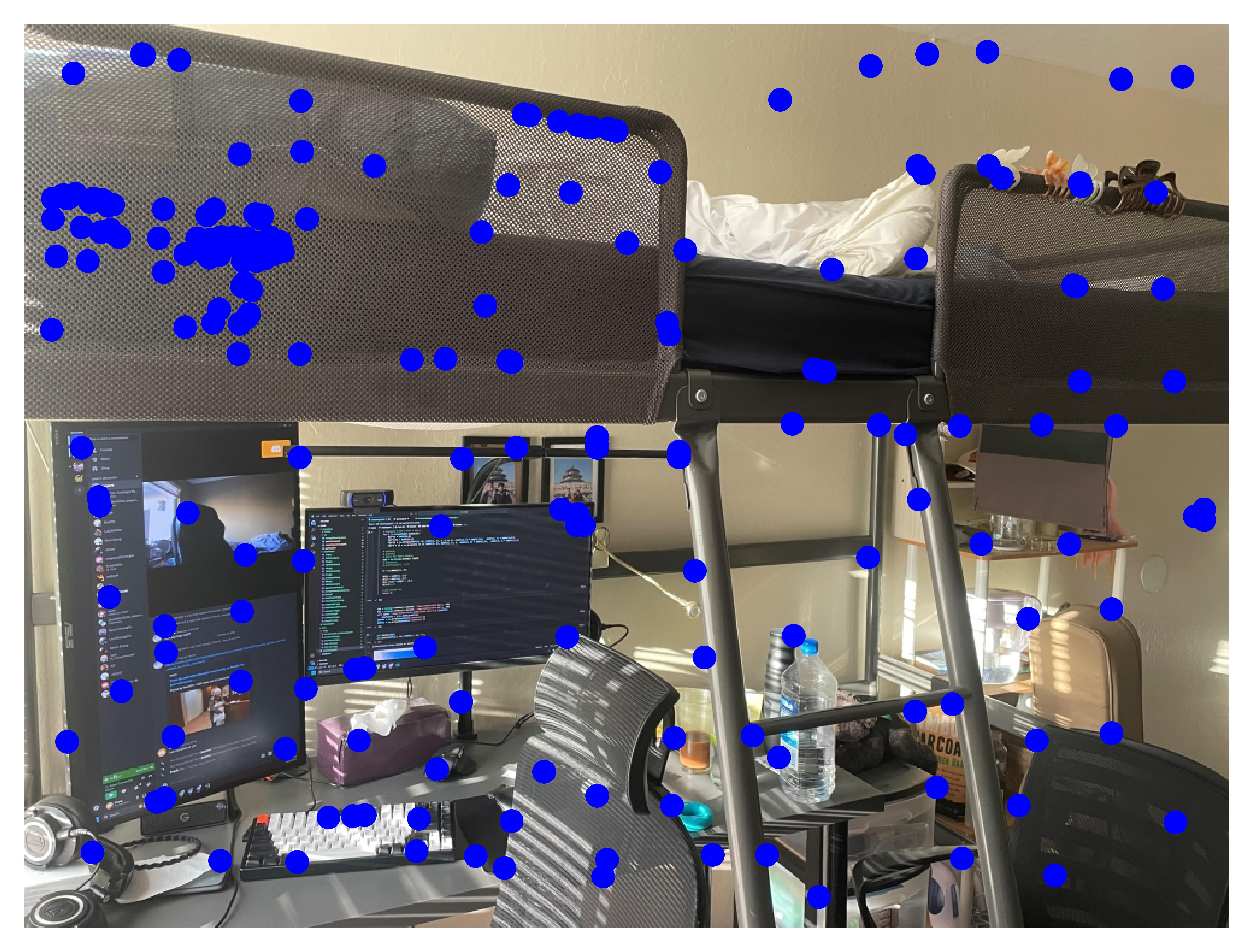
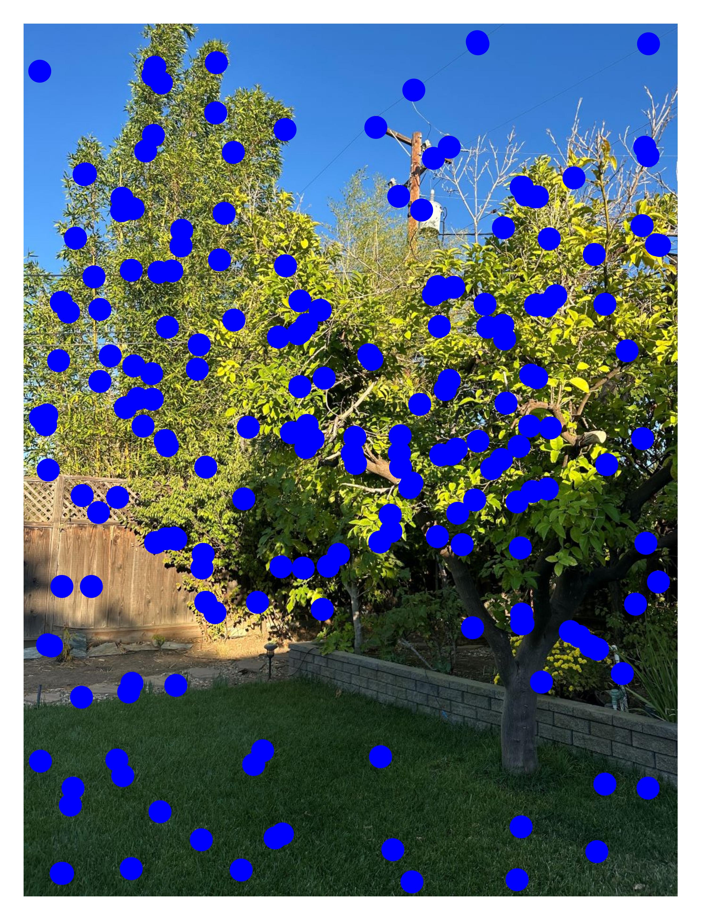
The first step of the process is to try to identify potential points of interest on the image. These would be things such as corners, since it lends itself to be more easily localized (as opposed to lines or surfaces). We use the Harris corner algorithm which computes the sum of products of gradient around a image patch, then using its eigenvalues to determine if its a line, edge, or surface. If both eigenvalues are small, then its probably a surface, if one is small -- a line, if both are large -- a corner. The result is a large set of potential interest points, which we need to further filter down.

You may see that no points are being picked at the very edge of the image. This is important when we create feature descriptors, as points on the edge would create very poor feature descriptors.

Harris Corners

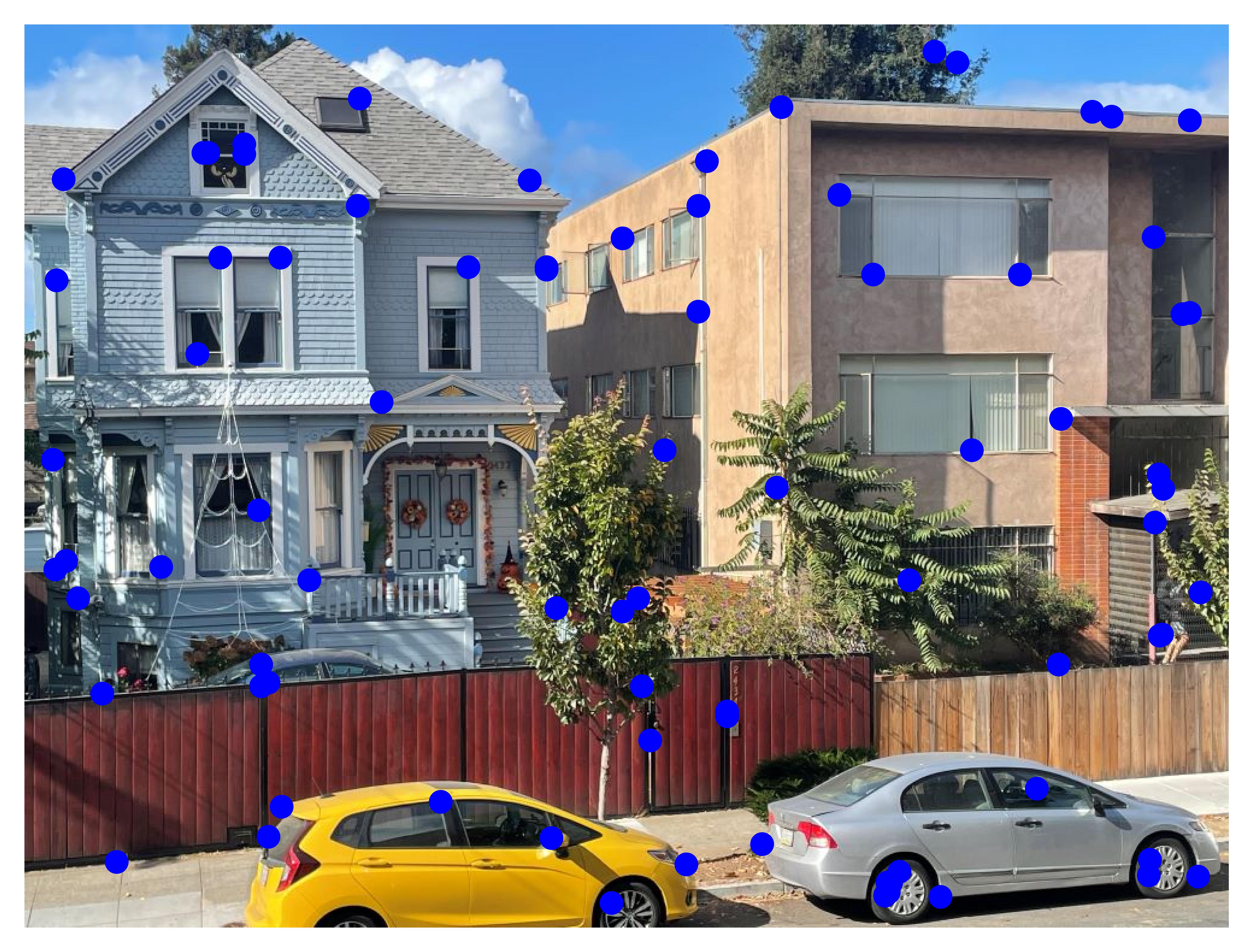
Adaptive non-maximal suppression

One method of filtering could be just taking the strongest corners in the list of Harris corners we obtained. However, this often leads to clusters of points, which would result in our homography to be very sensitive to noise. Instead we employ a technique called "Adaptive Non-maximal Suppression", which spreads out the interest points much better. In theory how this algorithm works is that it finds the smallest radius for each point, where another point in that radius has a significantly stronger corner. Then the points we use are the ones with the largest radius. This way we ensure a more even spread of points, and more points on weaker areas, less points on stronger areas. This helps with computing homography, as more points on weaker areas helps average out a good homography and makes it less sensitive to noise.

Im1 with 80 Points

Im2 with 80 Points

Keypoint Matching

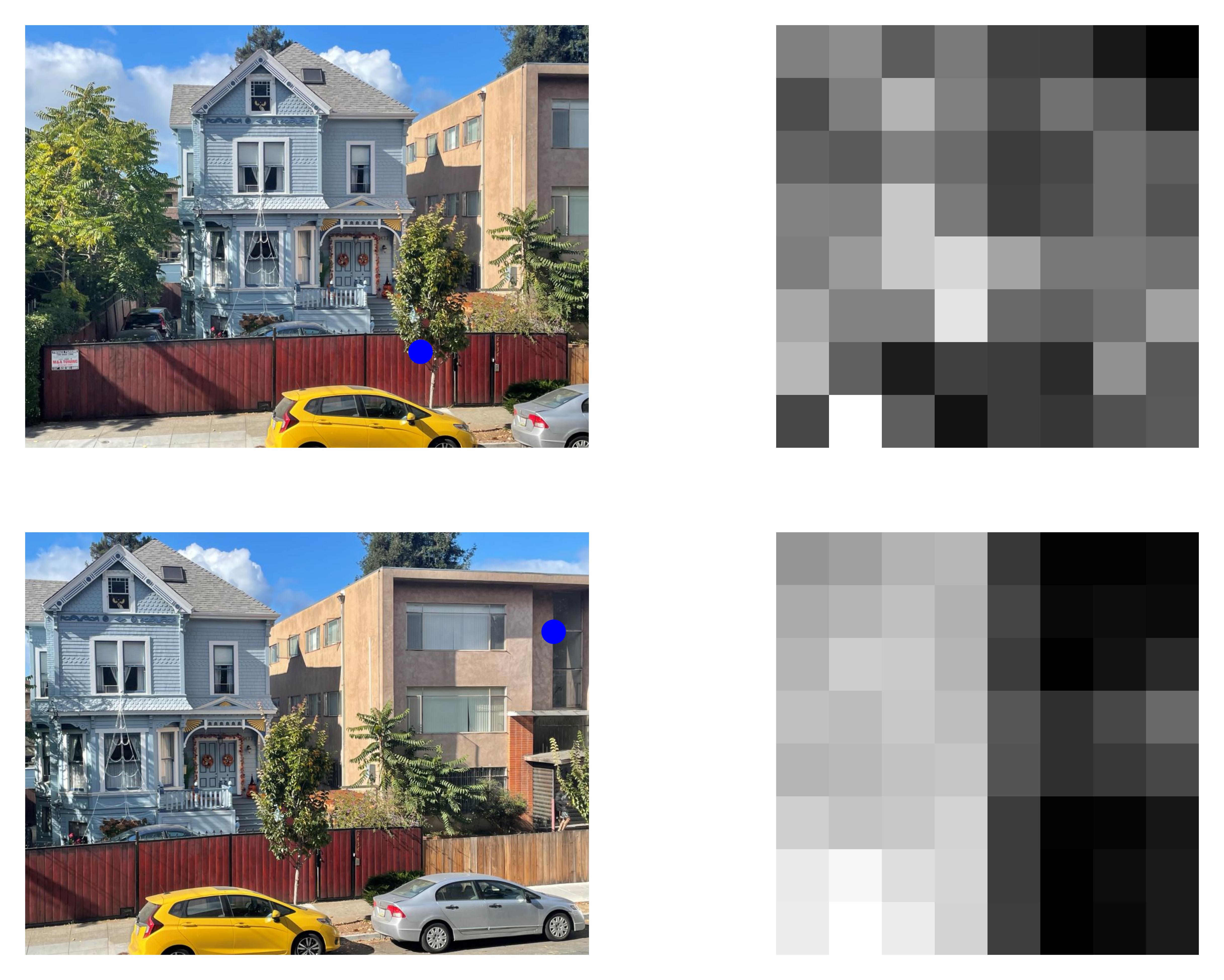
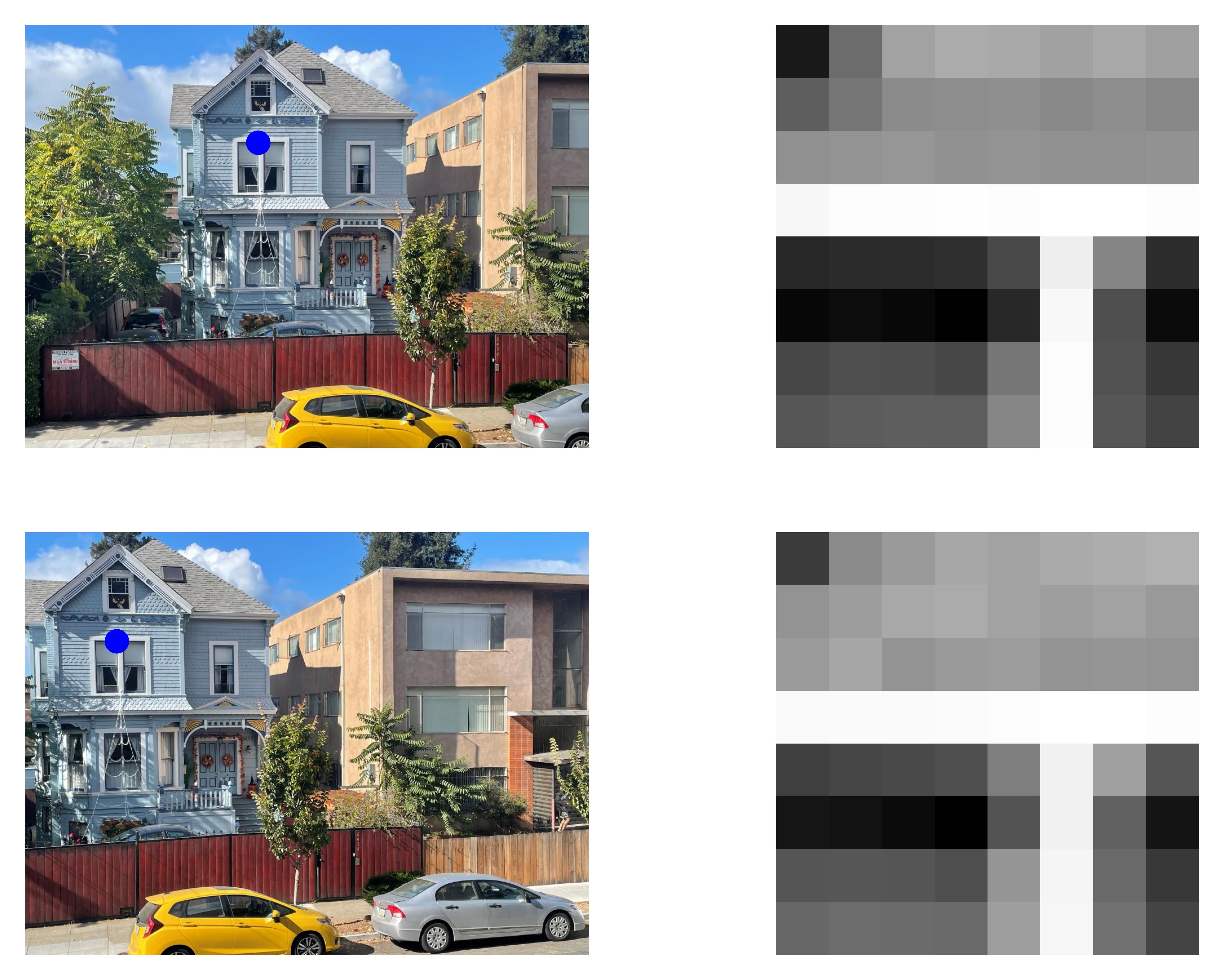
Now that we have our interest points on both images, we need a way to figure out correspondances. In other words, which pairs of points are on the same location on each image? To do this we first need a way to compare the area that the point is on. We can use a 8x8 descriptor sampled from a 40x40 box around each point. It is important each point is only sampled once to avoid aliasing. Another way to think about this process is that we are convolving an area with a mask, where the stride is the size of the mask. In this case we are convlving a 40x40 area with a 5x5 mask, with stride 5. This gives a blurred image that approximates the area around the point. Given two of these descriptors we can check how similar they are and decide if they are describing the same point.

Descriptors

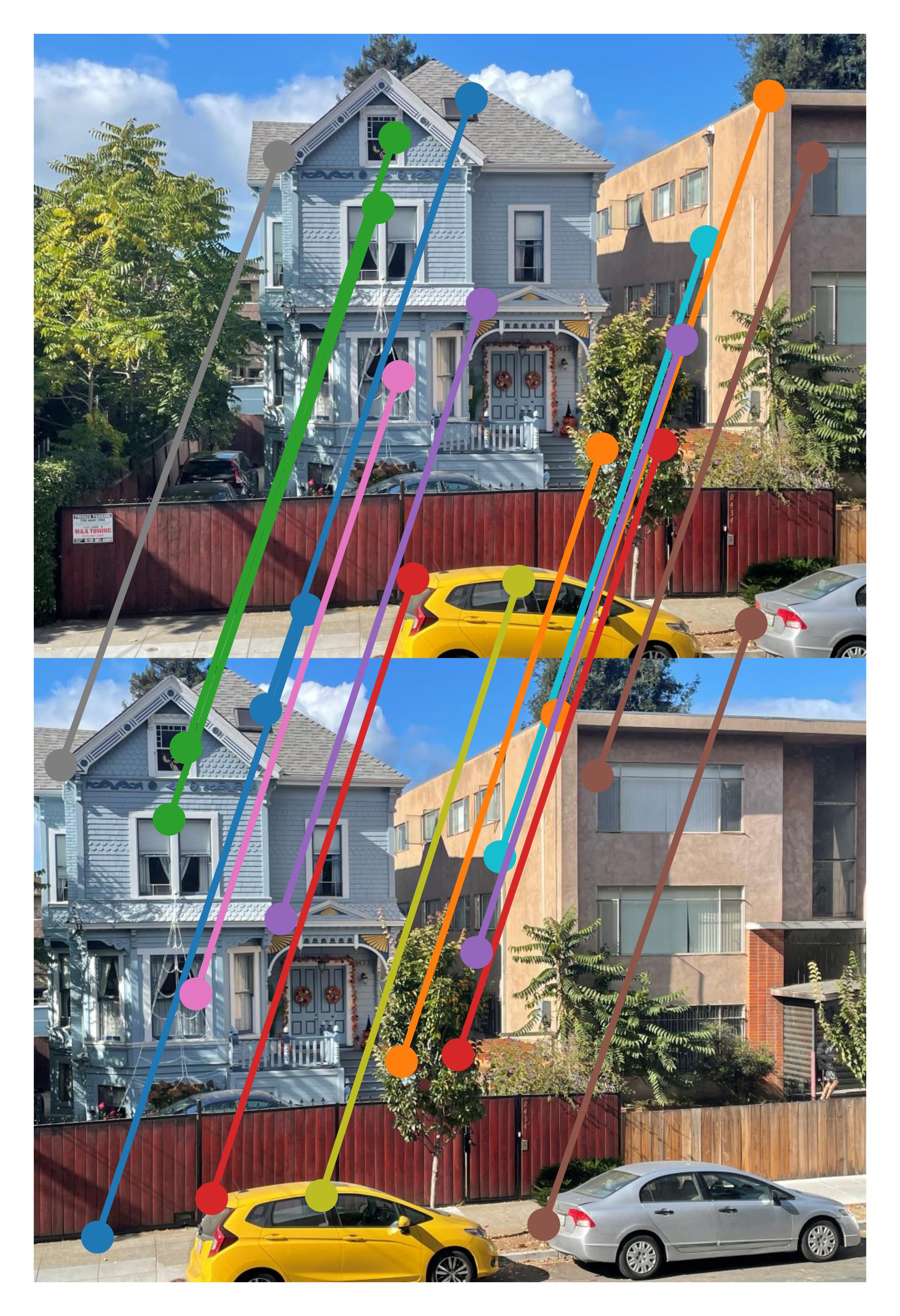
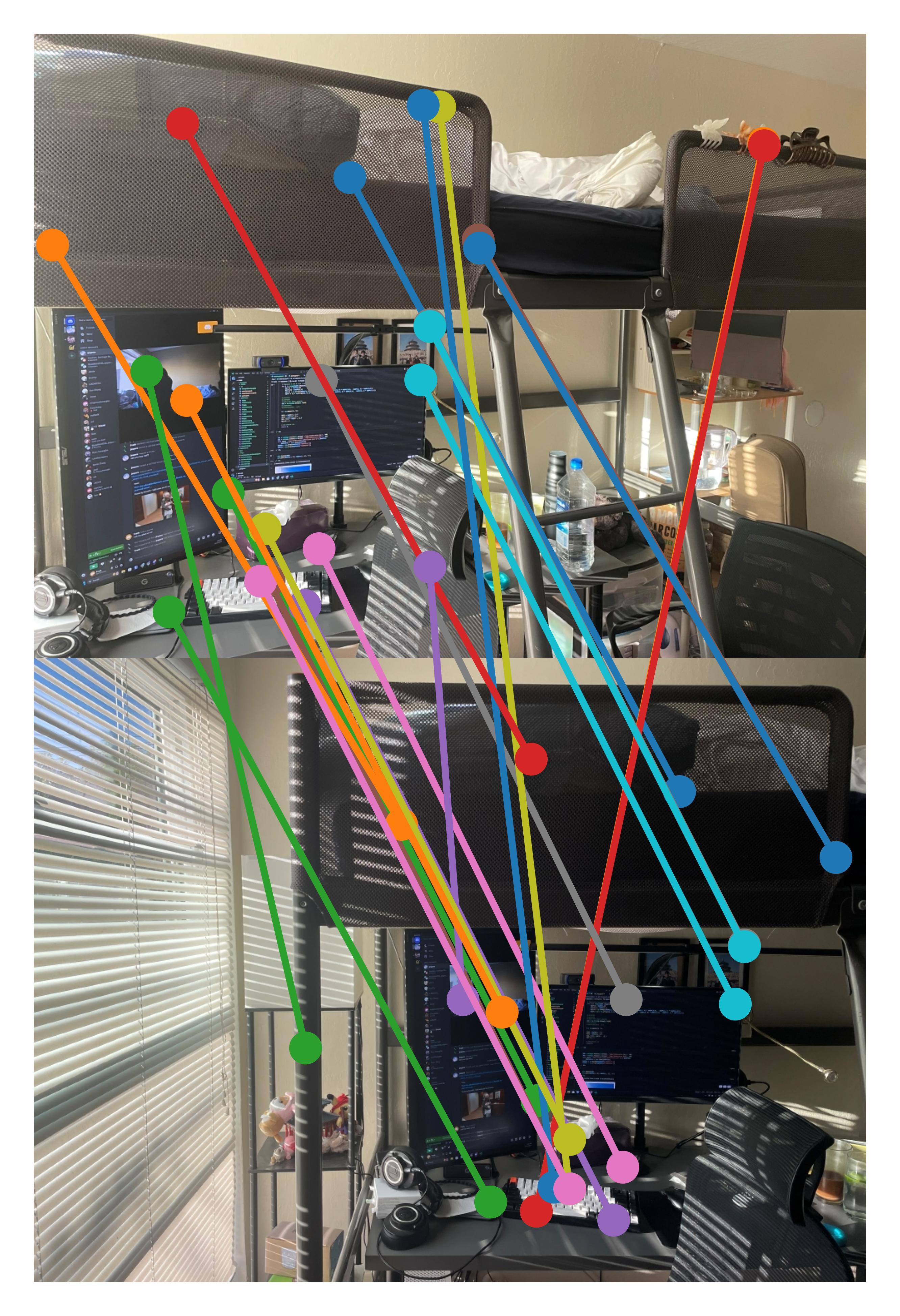
We can push the points of one image through a nearest-neighbor model and then find the nearest-neighbor of the points of the second picture. Here we use the Lowes rule to find points which have a fit that is much better than the rest. The ratio I used is 0.75, meaning the ratio of nn1/nn2 is less than 0.75. Using a higher ratio of 0.85 gave me mostly true positive values, although there were still a few false positives, but made alignment worse later on. Looking at their descriptors we can see why the model may have thought these points were similar.

True Positive

False Positive

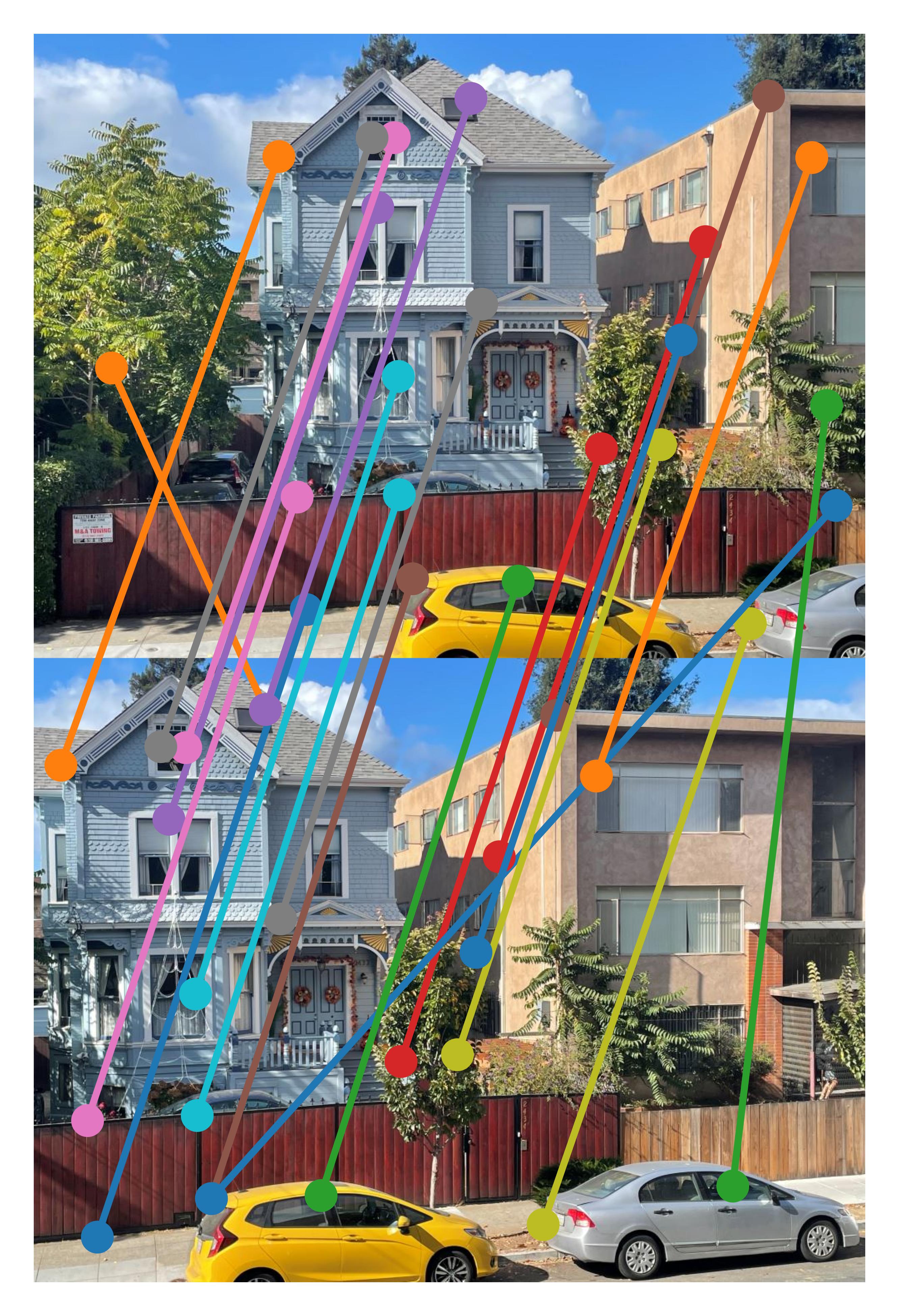
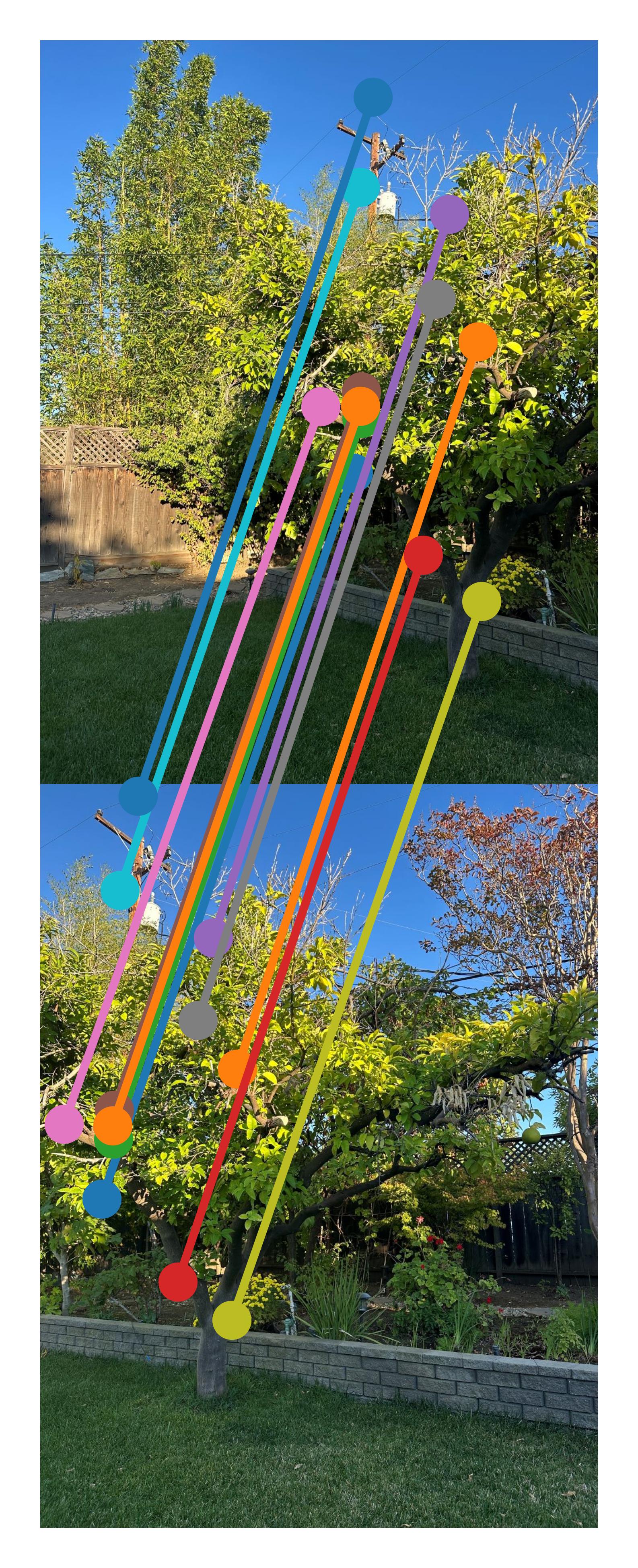
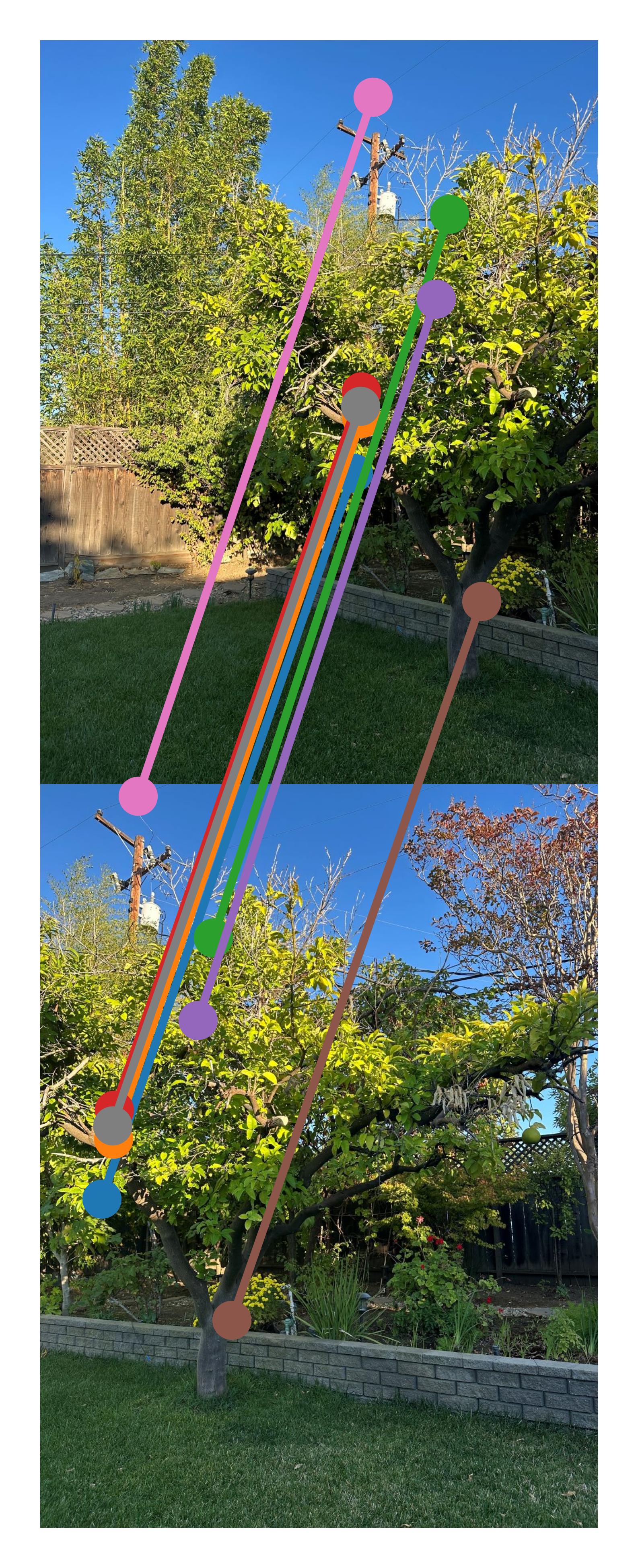
We can now match the points, giving us this result.

Lowes Ratio of 0.75

Lowes Ratio of 0.85

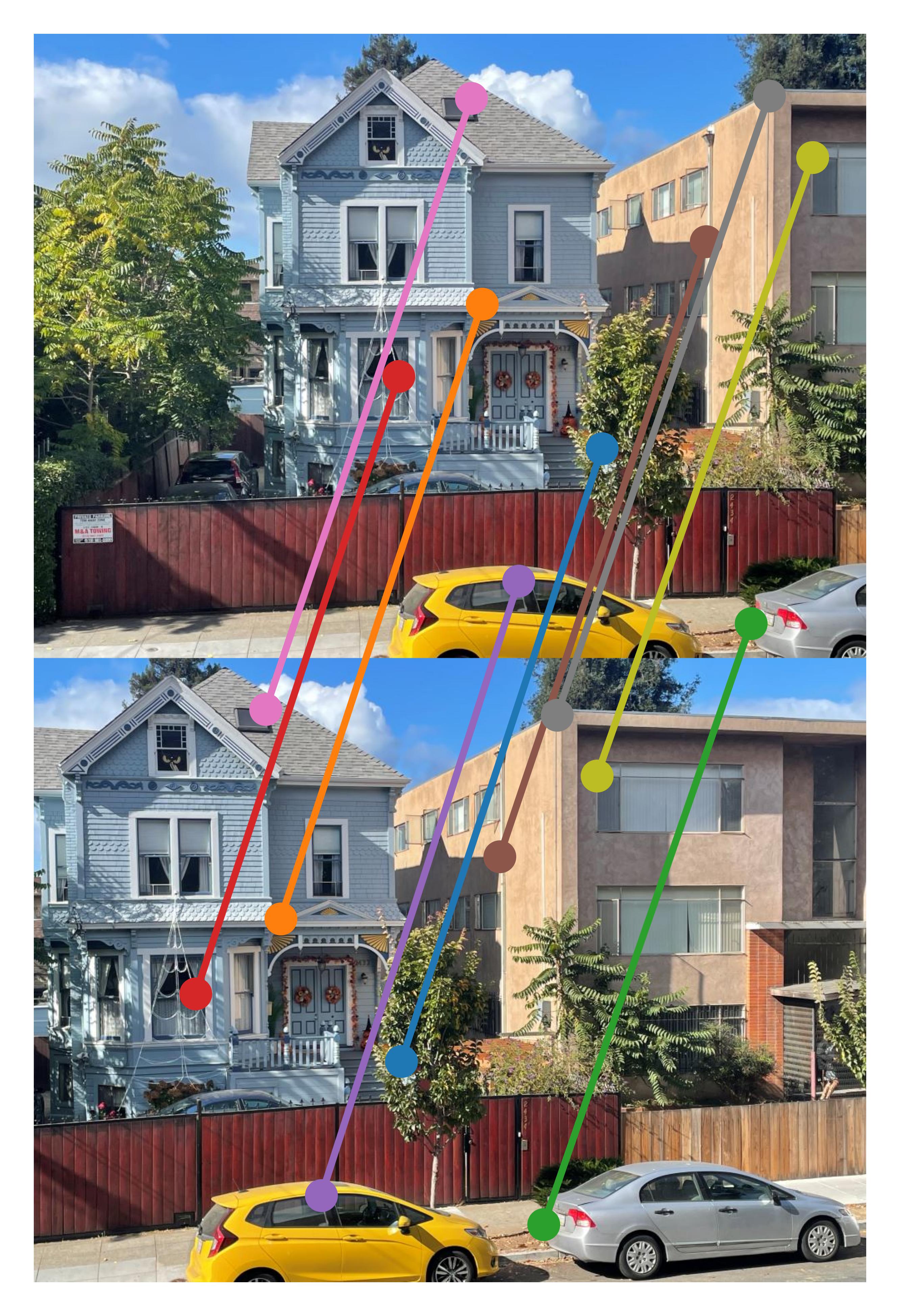
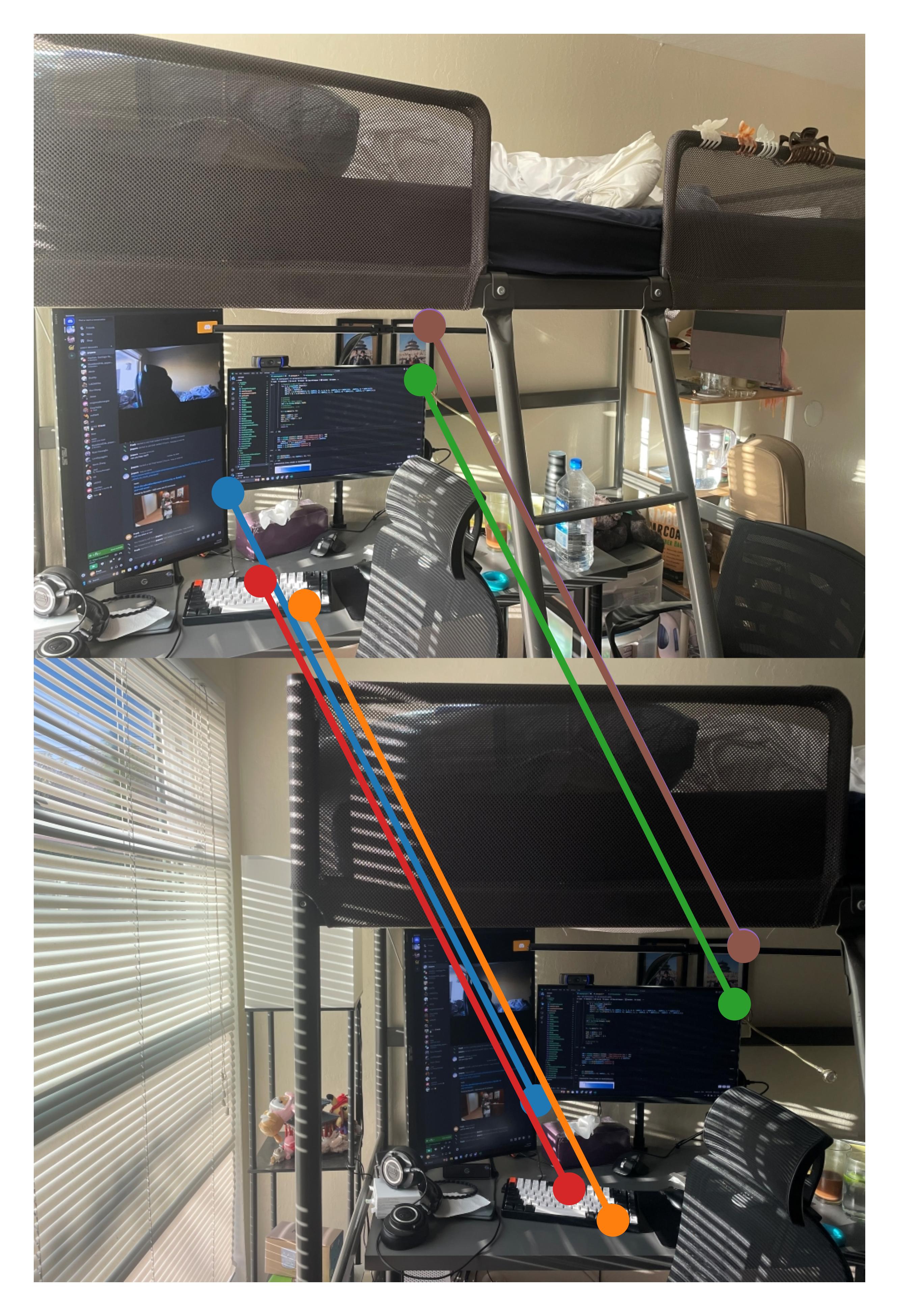
Another filtering step is done to both elimate outliers seen in the image above. This is done by RANSAC, where 4 points are randomly selected, their homography is calculated, and applied to the other points. If the resulting point is within a certain distance of the actual point (in this case I used 1 pixle), then it is an inlier, otherwise it is an outlier. After repreating this process a number of times, or until a certain percentage of points become inliers, we stop, and calculate the overall homography of all inliers. This elimates a few points and gives us the following result.

RANSAC Tolerance of 1

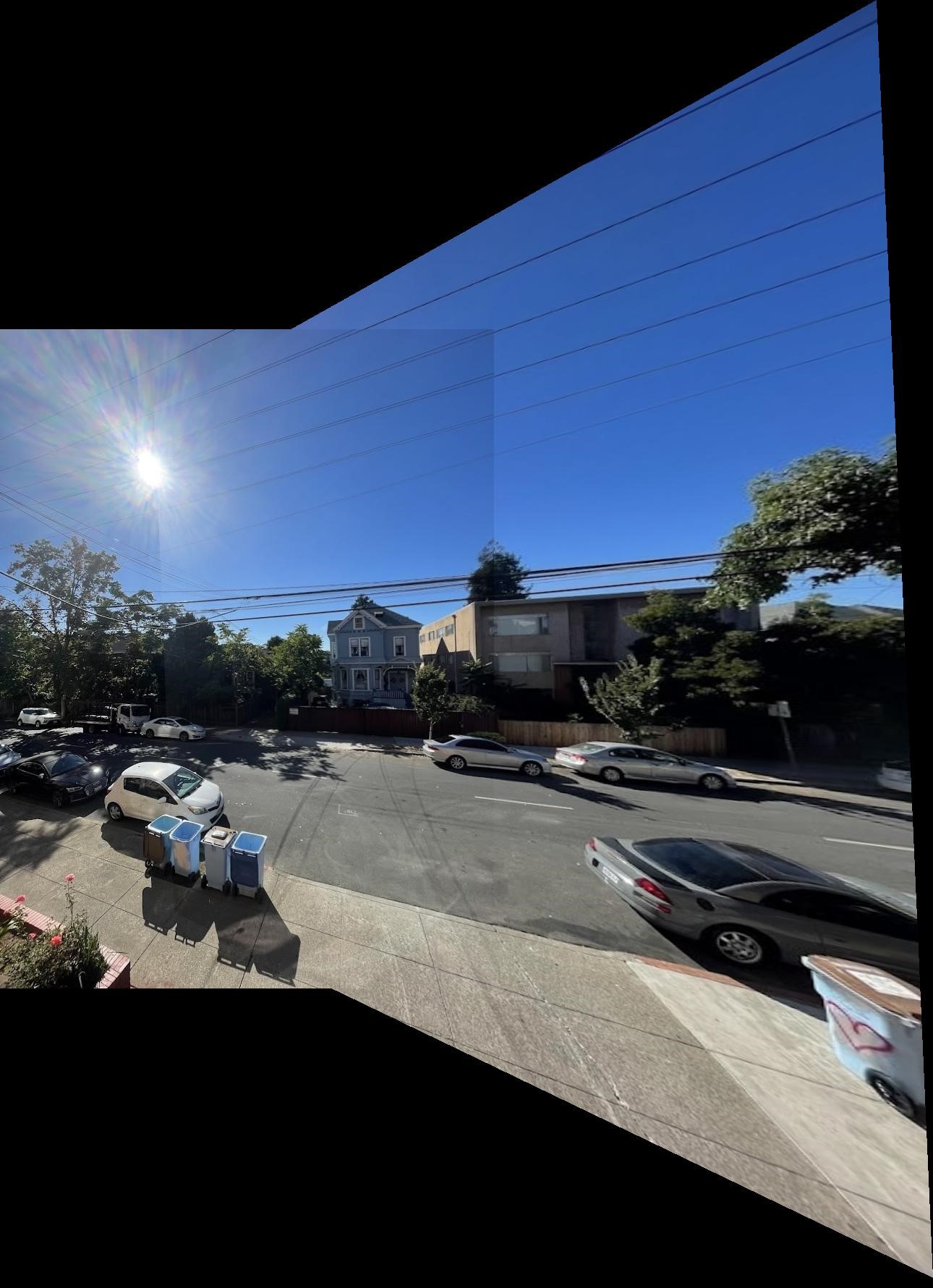
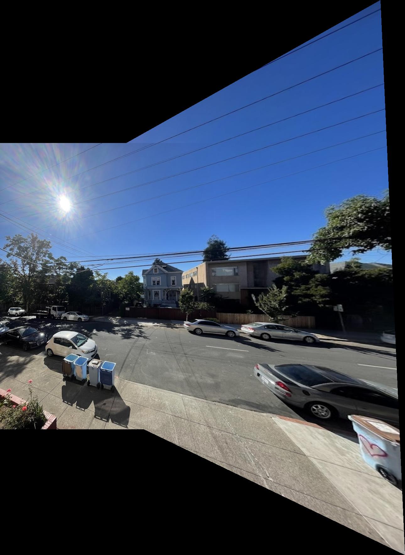
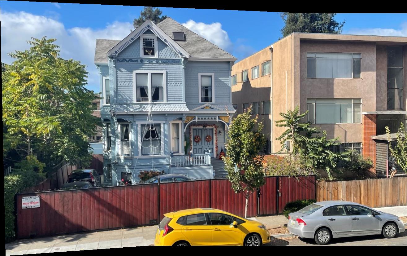
Finally, we take the homography and build the panoramic the same way as in the manual method.

Auto Point Selection

Manual Point Selection

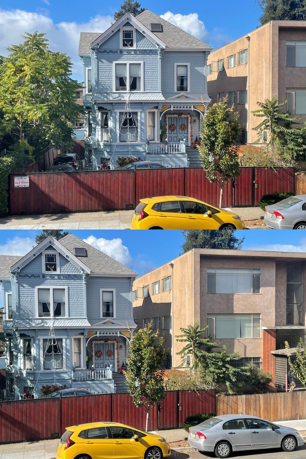
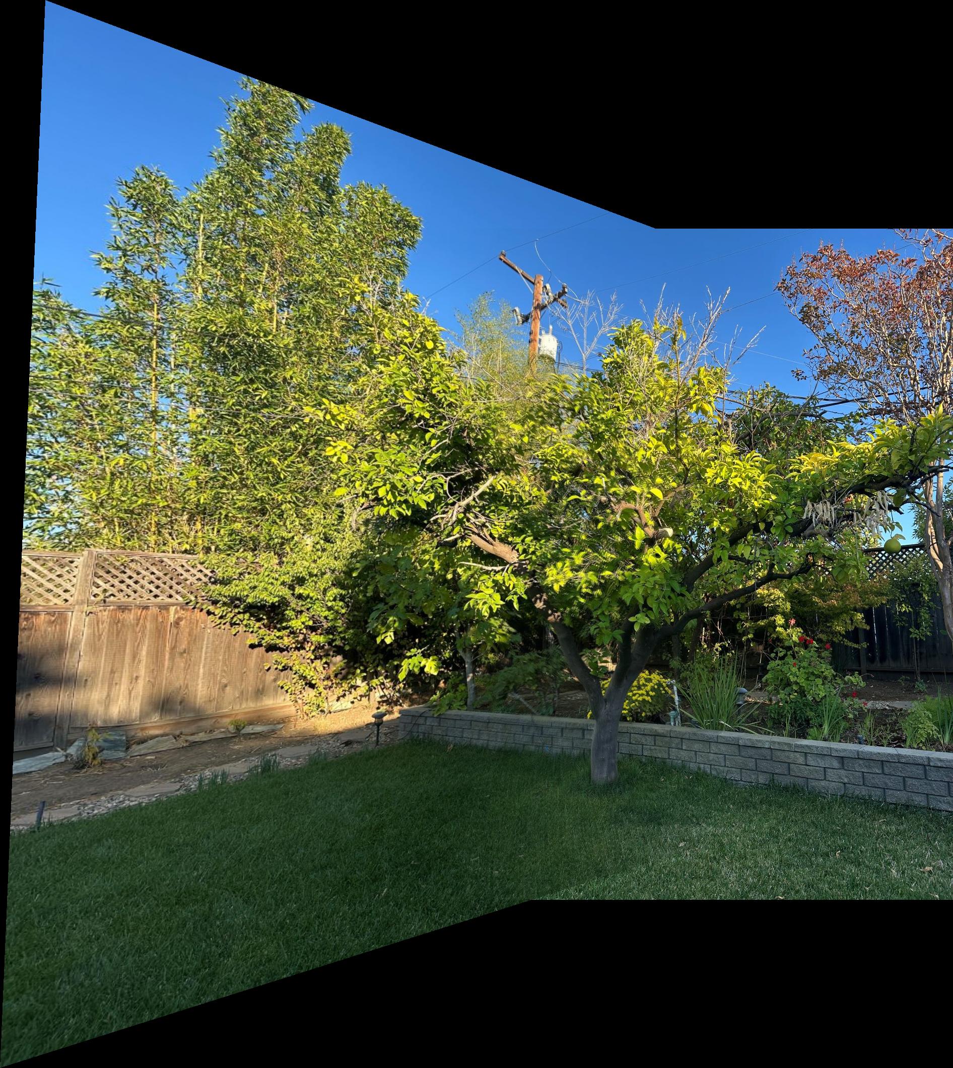
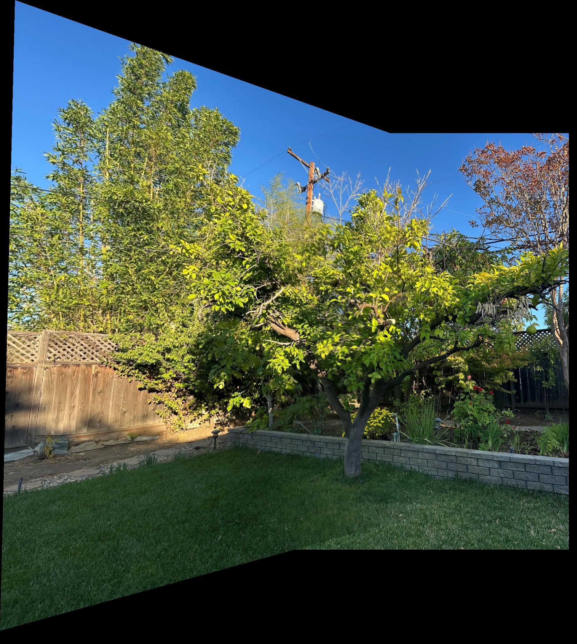
In the next image, manual selection did not have the x-coord blending done, but besides that you can see the results are almost the same.

AMNS

Keypoint Matching

RANSAC

Auto Point Selection

Manual Point Selection

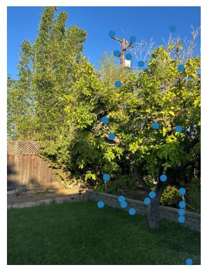
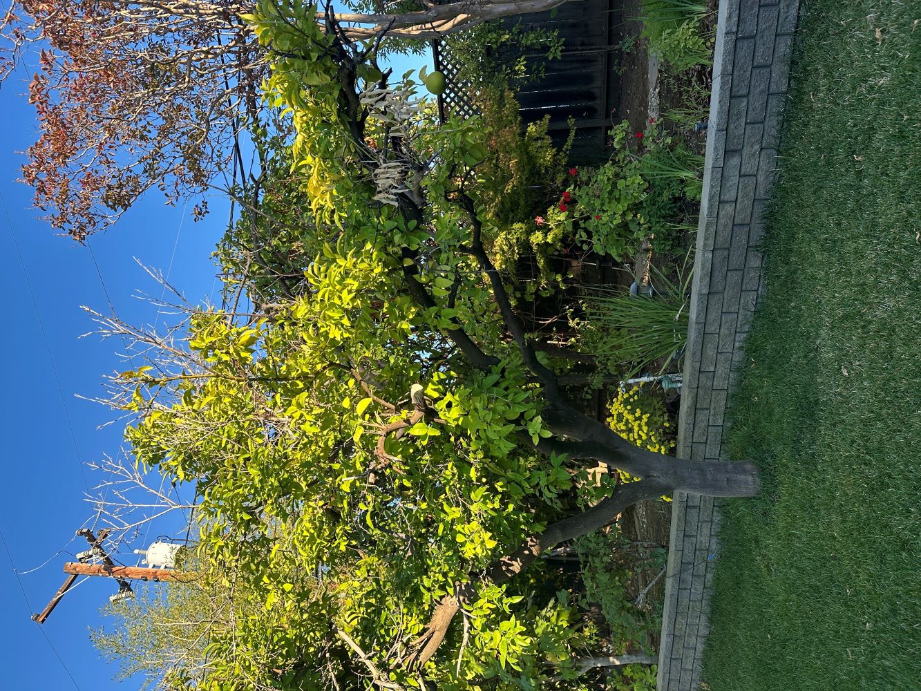
Finally, the auto panoramic process does quite well in the tree image. This is suprising as most of the image is featureless grass, and I had a hard time manually defining points.